As we have a MD trajectory of multiple PEO chains in a box, we must select each of them and then calculate their radius of gyration. This means that we have to create a .ndx file, which contains the index number of each constituent of PEO chain. This can be achieved easily using a python script. A file called `selection.ndx' was generated, which has the following content:
With this, a shell script can be written to generate a .xvg for each PEO chain in the box:
#!/bin/bash
for i in {0..19..1}
do
echo $i | gmx gyrate -f md.trr -s md.tpr -n selection.ndx -o r$i.xvg
done
This will generate a series of files, such as r0.xvg, r1.xvg ... r19.xvg. Each of these .xvg files contains root-mean-square value of the radius of gyration at each time step. These values can then be averaged. In this calculation, it was found that the root-mean-square radius of gyration of PEO chain is $1.745~\mathrm{nm}$.
With the MD trajectory of PEO chains, the van hove function can easily be generated with the following command:
In the file van_hove.xvg, the van hove function $G(r,t)$ is expressed in the real space. It can be easily transformed to the fourier space, using the following:
\begin{equation}
\hat{G}(k,t)=4\pi\int_0^{\infty}\frac{\sin(kr)}{kr}G(r,t)r^2dr
\end{equation}
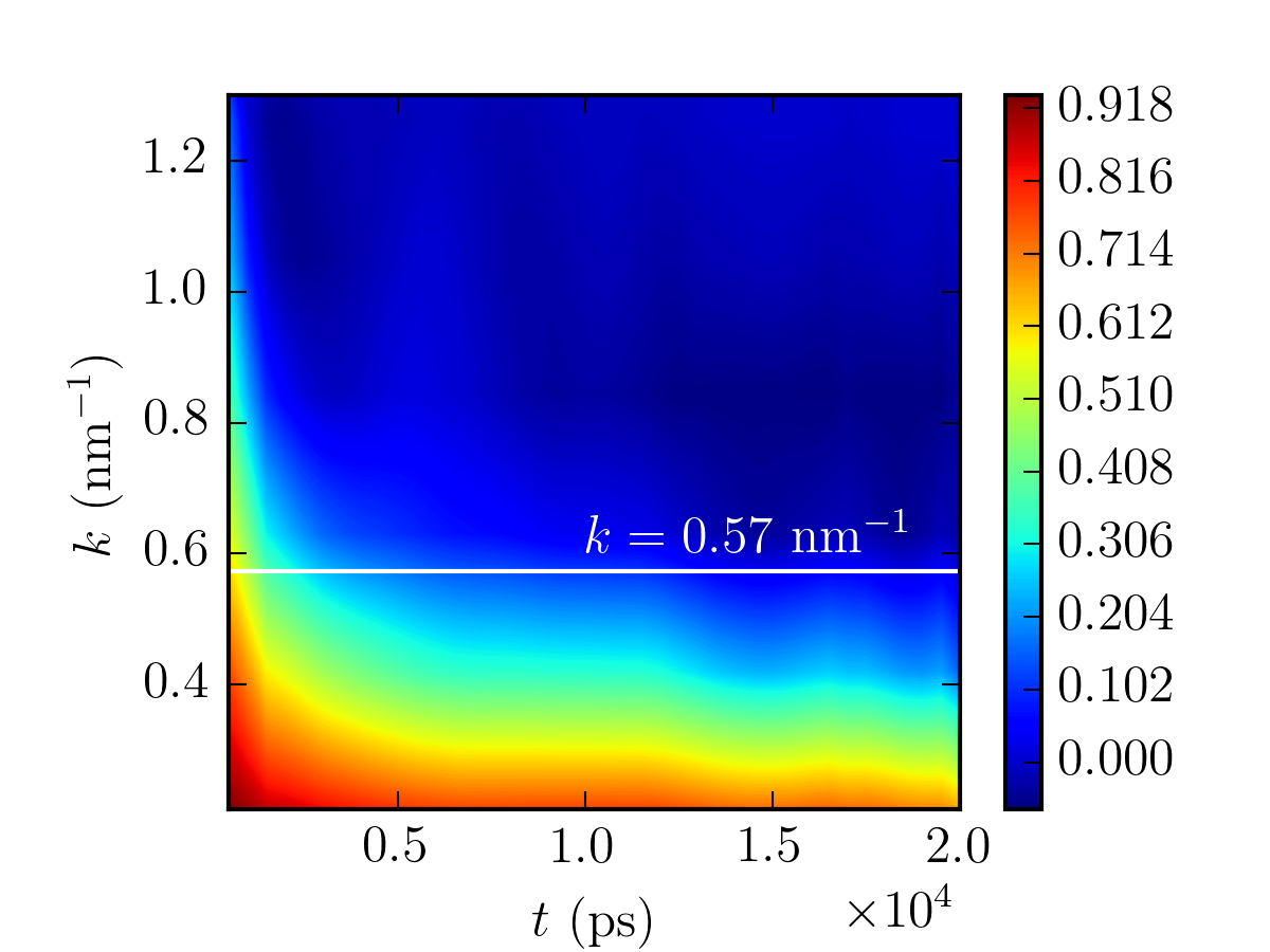
The van hove function is the time-dependent part of the dynamic structure factor, which tells us the probability of a particle having moved for a distance $r$ in a duration of $t$. When it is expressed in the fourier space, the relaxations of the chains at different length scales are revealed. The van hove function in fourier space has a maximum value of one and a minimum value of zero, which means 'not fully relaxed' and 'fully relaxed', respectively. For instance, from the MD trajectory of a polyethylene oxide melt, the van hove function can be calculated and transformed into the fourier space as shown in the contour plot of Figure 1. When $k\rightarrow 0$, where $k$ is the magnitude of the wavevector, it corresponds to the long length scale motion and vice and versa. The contour plot shows that when $k$ is small, the colour of the contour plot is mostly red in color, meaning that the motion is slow and the chains are not fully relaxed; as $k$ becomes large, the color of the contour plot turns blue in color, which indicates fast motion of the segments of chains. This contour plot allows us to extract transport properties of the polyethylene oxide melt, and to check how relaxed the system is.
For instance, in this case, the root-mean-square radius of gyration of PEO chain is $1.745~\mathrm{nm}$. A line at $k=1/1.745=0.57~\mathrm{nm^{-1}}$ is drawn on the contour plot, which corresponds to the long length scale motion of the chain. Along the line, the height of the surface is almost zero, indicating that the system is relaxed.
Figure 1: The van hove function of polyethylene oxide melt in fourier space. When $k$ is small, it corresponds to the long length scale motion of the chain, and vice and versa for the longer wavevector.
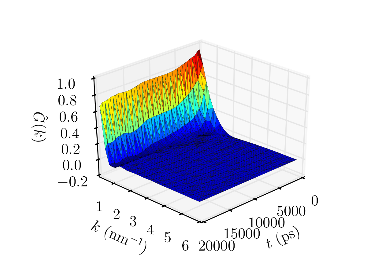
Figure 2: A 3D plot of the van hove function of polyethylene oxide melt in fourier space.